- Ruhr-Universität Bochum

Atomistics Meets Statistics
The evolution of a metallic or multiphase microstructure during solidification or mechanical deformation largely depends on the structure and energy of the interfaces in the material. So do the resulting macroscopic properties, like the deformability, thermal stability, and strength. Consequently, substantial scientific effort is made to investigate grain boundary properties, and a valuable tool to do so are high-throughput atomistic simulations.
Nowadays high-throughput numerical simulations are standard in materials development, because they allow a systematic variation of material or process parameters. The most common approach to cover a broad range of these parameters in a short time is based on a regular, i.e. equidistant sampling of the parameter space, which keeps the automatisation of the workflow fairly simple. It has limited use however, when the properties of interest depend on several variables at the same time, i.e. a multidimensional parameter space has to be sampled, and the property of interest does not vary homogeneously in this space. This is the case for the energy of grain boundaries, which depends on the five macroscopic geometric degrees of freedom of the interface, defined by the rotation axis and angle and the inclination of the grain boundary plane, and exhibits deep local minima, so-called cusps.
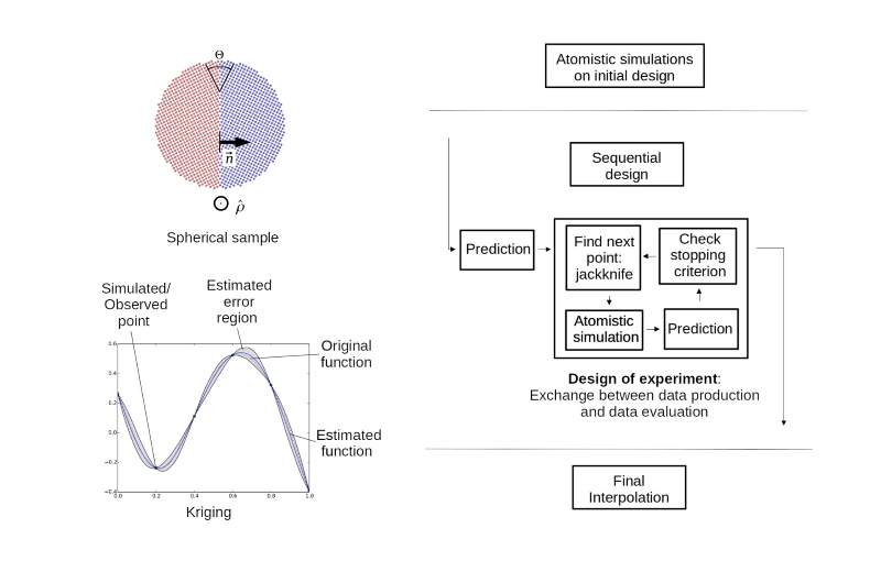
For such cases a sequential design of experiment (DOE) can be beneficial, during which the next points in the parameter space to be sampled are chosen based on the already available data (see Figure above).
The first important building block of the numerical recipe is the atomistic representation and optimisation of the grain boundary structure starting from the macroscopic degrees of freedom, and the calculation of the grain boundary energy. If the sampling scheme shall be valid for the complete 5D parameter space, including small angle and other general grain boundaries, the main challenge is to realise such a calculation without periodic boundary conditions. This can be achieved by using a spherical sample. The two half-spheres can be cut and oriented to represent any desired combination of misorientation axis, rotation angle, and plane inclination. By evaluating only the atoms in the interior of the sphere, surface effects are excluded.
After creating a first set of structure-energy data with atomistic simulations, a suitable interpolation method is required. The so-called Kriging (also referred to as Gaussian process regression in the presence of noisy observations) predicts the value of a function at a given point by computing a weighted average of the already determined values of the function in the neighborhood of the point. This approach is related to a regression analysis, but Kriging exactly interpolates through the existing observations. Furthermore, it provides a natural measure of uncertainty quantification for predictions at potential locations. In the sequential design, this information is used to create a list of candidate points for new sampling locations from the regions where the uncertainty is maximal. In these regions the points with the maximum expected variance compared to their neighbors will be chosen, in other words, points which are expected to be on a steep slope in the energy landscape.
A typical sequence of experiments for a one-dimensional example – the energy of symmetrical tilt grain boundaries as a function of misorientation angle – demonstrates the advantage of the sequential design, namely that cusps which are not included in the initial data are identified by the algorithm after a few steps only. This is particularly advantageous for more complex subsections of the 5D parameter space. The energy minima for different inclinations of the plane (given by the two angles that define the normal vector of the plane) of a small-angle grain boundary cannot be easily predicted from crystal symmetry but are revealed by the DOE algorithm. The underlying strategy will be advantageous for any application with strong, localized fluctuations in the values of the unknown function.
